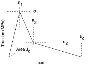
Trilinear Traction Law
The Traction Law
This traction law assumes a piece-wise linear relation with two arbitrarily-specifiable break points (i.e., three linear pieces). There are separate traction laws for opening displacement (mode I) and sliding displacement (mode II).
The toughness is
[math]\displaystyle{ J_c = {1\over2}\bigl(\sigma_1\delta_2 + \sigma_2(\delta_c-\delta_1)\bigr) }[/math]
The traction law for each mode depends up seven properties - (δ1,σ1) and (δ2,σ2) breakpoints, critical COD (δc), total area or toughness (Jc), and the initial elastic slope (k). You must enter exactly 5 of these seven properties for each mode. Furthermore, if one of the 5 is the initial slope, then δc along with either σ1 or δ1 for that mode (but not both) must be among the specified properties. The two remaining unspecified parameters will be calculated from the five provided parameters. The final law must satisfy 0 < δ1 ≤ δ2 ≤ δc, δc > 0, σ1 ≥ 0, σ2 ≥ 0, and σ1+σ2 > 0. Note that these restriction prohibit infinite initial stiffness (i.e., δ=0) but allow zero initial stiffness (i.e., σ1=0). It is not clear if zero initial stiffness has any realistic applications.
One useful interpretation of a trilinear law is that it is modeling two physically mechanisms. The total toughness is the total area under the curve and is given above. The first failure mechanism can be identified with the area under the first peak and bounded by the dotted red line in the above figure. This partial area is the toughness for the first mechanism and is equal to
[math]\displaystyle{ J_1 = {1\over2}(\sigma_1\delta_2 - \sigma_2\delta_1) }[/math]
The remaining area is associated with the second mechanism. Its toughness is equal to
[math]\displaystyle{ J_2 = {1\over2}\sigma_2\delta_c }[/math]
For example, the first peak might be associated with crack tip fracture toughness while the tail models a process zone such as fiber bridging. In fact, in the limit as σ1 → ∞ and δ2 → 0, a simulation with a pre-existing cohesive zone should approach a simulation propagating a crack tip using fracture mechanics along with a linear softening traction law having σ2 as the cohesive stress. NairnMPM can do both these simulations and the results will be similar. The pure cohesive zone simulation is done by using a trilinear traction law on an existing crack. The combined fracture mechanics/cohesive zone simulation starts with a crack that propagates when energy release rate at the crack tip is equal to J1. Furthermore, the crack propagation commands are set to leave a cohesive zone in the wake of the crack. This cohesive zone can be a |triangular traction law with its toughness equal to J2 and stress equal to σ2. Both these types of simulations are described in Nairn (2009).[1]
Failure
This laws uses uncoupled mode I and mode II cohesive laws. The failure is handled by the same methods used for the Triangular Traction Law. This cubic cohesive law can also be used for mode I or mode II laws in coupled mixed-mode modeling[2] by using the Mixed Mode Traction Law.
Traction Law Properties
The following properties are used to create a trilinear traction law:
| Property | Description | Units | Default |
|---|---|---|---|
| sigmaI2 | The stress at the second break point (σ2) in mode I or opening mode | pressure units | none |
| sigmaII2 | The stress at the second break point in mode II or sliding mode | pressure units | none |
| delpkI2 | The relative COD at the second break point in mode I or opening mode; it is equal to δ2/δc | dimensionless | none |
| delpkII2 | The relative COD at the second break point in mode II or sliding mode; it is equal to δ2/δc | dimensionless | none |
| (first point) | Use the triangular traction law properties to enter the first break point COD and initial slope for each mode | varies | varies |
| (other) | Properties common to all traction laws, where sigmaI and sigmaII apply to the first break point stress | varies | varies |
