LoadControl Custom Task

A custom task run a load control simulation based on calculations of contact or reaction forces.

Introduction

This CustomTask tries to achieve the load requested from a provided user defined function by adjusting the velocity of a block of rigid material points. The control is done using a non-linear PID control algorithm.

Specifying the Force

A LoadControl custom task is based on a block of RigidBC or RigidContact particles. These particles are typically placed on the edge of the specimen. The following steps are used to setup all simulations with load control. First pick a direction as 1, 2, or 3 for x, y, or z direction. Load control is limited to be along grid axes. Next create rigid particles to apply the load:

1. Define a RigidBC material to control velocity is the specified direction or define a RigidContact material. Do not use any setting functions in the rigid material definition.
2. Place a block of those material points using that defined rigid material on the edge to be loaded.
3. Include displacement of the defined rigid material in the global archive using dispx, dispy, or dispz for the chosen direction.
4. When using RigidBC particles, include reaction force for the defined rigid material in the global archive using reactionx, reactiony, or reactionz for the chosen direction.
5. When using RigidContact particles, include contact force for the defined rigid material in the global archive using contactx, contacty, or contactz for the chosen direction.
6. Choose global archiving time to provide stable load control

Start the custom task and define the following force defining parameters

CustomTask LoadControl
Parameter direction,(loaddir)
Parameter material,(matID)
Parameter matname,(matname)
Parameter load,(loadfunction)

where

• (loaddir) is 1, 2, or 3 for x, y, or z direction loading.
• (matID) or (matname) is the defined rigid material by number or name.
• (loadfunction) is a user defined function that defines desired load (in force units) as a function of time (in alt time units)

Non-Linear PID Control

The control loop starts by estimating the error in current displacement using

      [math]\displaystyle{ e = \frac{F - L(t)}{A_t} }[/math]

where [math]\displaystyle{ F }[/math] is the rigid material reaction or contact force in the global archive, [math]\displaystyle{ L(t) }[/math] is the desired load from the Load parameter function, and [math]\displaystyle{ A_t }[/math] is the tangent stiffness for rigid material force (in force units) per unit displacement (in displacement units). If [math]\displaystyle{ A_t }[/math] is constant, the control is a linear PID. But for many simulations, such as those with plasticity, damage, or non-linear elasticity, [math]\displaystyle{ A_t }[/math] will evolve during the simulation leading to non-linear PID. The PID algorithim changes the rigid material points velocity in the control direction to

      [math]\displaystyle{ v = \frac{1}{t_g}\left(K_pe + \frac{K_i}{t_g}\int_0^t e\thinspace d\tau + K_dt_g\frac{de}{dt}\right) }[/math]

where [math]\displaystyle{ K_p }[/math], [math]\displaystyle{ K_i }[/math], and [math]\displaystyle{ K_d }[/math] are dimensionless gain factors for proportional (P), integral (I), and derivative (D) errors and [math]\displaystyle{ t_g }[/math] is the simulation's global archiving time.

Selecting PID Control Parameters

Load control depends on global archiving time [math]\displaystyle{ t_g }[/math], [math]\displaystyle{ A_t }[/math] (and how it evolves), [math]\displaystyle{ K_p }[/math], [math]\displaystyle{ K_i }[/math], and [math]\displaystyle{ K_d }[/math]. In addition, reaction and contact forces on rigid materials are typically noisy meaning that some of the control variables will require smoothing for stable control. All relevant parameters are set with the following commands:

Parameter velocity,(initvelocity)
Parameter minVelocity,(minvelocity)
Parameter startupTime,(inittime)
Parameter At,(initAt)
Parameter smoothF,(smoothF)
Parameter smoothA,(smoothA)
Parameter smoothErr,(smoothErr)
Parameter Archive,(stubwext)
Parameter Kp,(Kp)
Parameter Ki,(Ki)
Parameter Kd,(Kd)

Methods to choose these parameters are in the following sections.

Choosing Start Up Conditions

To get started, a load control task needs an initial velocity and an initial stiffness [math]\displaystyle{ A_t }[/math] (which is required to calculate control error). Furthermore, reaction and contact forces in dynamic calculations take a while to settle into reasonable values (such as when loading at constant velocity). A load control task thus normally needs a (inittime), which is a time over which the rigid particles move at constant (initvelocity) without imposing any control. Once the start up time has passed, the load control begins using an initial [math]\displaystyle{ A_t }[/math] that can be determined one of two methods:

1. If you do not want to (are not able to) calculate an initial [math]\displaystyle{ A_t }[/math], specify a positive (inittime). The initial [math]\displaystyle{ A_t }[/math] will be found by least squares slope for force vs. displacement up to (inittime). Any provided (initAt) will be ignored. Note that this methgod cannot be used if (initvelocity) is zero.
2. Specified [math]\displaystyle{ A_t }[/math]: If you can calculate initial stiffness for the simulation, you can enter it in (initAt) parameter and then set (inittime) to minus the desired start up time. Once the time is passed, control will start with the provided [math]\displaystyle{ A_t }[/math].

Finding [math]\displaystyle{ A_t }[/math] from slope of force vs. displacement requires that (inittime) be 10-20 multiples of [math]\displaystyle{ t_g }[/math] to have enough points to fit a line. The start up time must also be long enough that the calculation is not adversely affected by dynamic start-up artifacts. Even when specifying [math]\displaystyle{ A_t }[/math] with negative start up time, the time should be long enough to bypass dynamic start-up artifacts. If control is started too soon, those artifacts may lead to unstable results.

During control steps, the value of [math]\displaystyle{ A_t }[/math] is continually adjusted to the current tangent modulus that is given by

      [math]\displaystyle{ A_t = \frac{F_t - F_{t-1}}{v t_g} }[/math]

If the velocity gets too low (which is expect if control is seeking constant force), this calculation will become unreliable (the denominator will be too small). To avoid unreliable updates to [math]\displaystyle{ A_t }[/math], this calculation can be limited to control steps for which velocity magnitude is greater than absolute value of input (minVelocity) (if no minimum input is provided, the default is to use 5% of (initVelocity)).

Choosing Smoothing Parameters

Reaction and contact forces recorded in global archives are typcially noisy. To avoid this noise from adversely affecting load control calculations, it is usually necessary to smooth some load control parameters. All smoothing is done by exponential smoothing with smoothing parameters from 0 for no smoothing to 1 for complete smoothing (i.e., the result remains fixed at initial value). The three smoothing options are

1. smoothF - smooth recorded reaction or contact force. This smoothing is probably always required. If no input value is provided, the default value is 0.9. This smoothing is limited to the interval [0,1) (i.e., 1 is not allowed).
2. smoothA - if dyanamic updates to [math]\displaystyle{ A_t }[/math] are noisy, the updates can be smoothed. This parameter can use the entire iterval [0,1]. A value of 1 means [math]\displaystyle{ A_t }[/math] will remain fixed in the initial value. Note that a fixed [math]\displaystyle{ A_t }[/math] turns this task in a linear PID control algorithm. That approach, however, may not work well for problems where stiffness changes do to effects such as plasticity, damage, or non-linear elasticity. Such problem require non-linear PID with evolving [math]\displaystyle{ A_t }[/math] otherwise control parameters based on linear PID may become unstable.
3. smoothErr - smooths the e(t) calculation. The default value is zero. This smoothing is limited to the interval [0,1).

Archiving Load Control Deetails

When using load control, especially when selecting parameters as explained in sections below, it is useful to archive load control results. To include archived results for a simulation, use the Archive parameter and set (stubwext) to a partial name with extension, such as "LC.txt". When this parameter is used, load control results will saved to a file with (stubwext) appended to the root path name defined for the simulation. The file will be a tab-delimited file for with time in the first column and the remaining columns having

     [math]\displaystyle{ A_t, \quad e, \quad \frac{1}{t_g}\int_0^t e\thinspace d\tau, \quad t_g \frac{de}{dt}, }[/math]

velocity set by the control algorithm, and smoothed force used in calculations. The file will begin with comment lines (lines starting in "#") that describe the load control parameters being used.

Choosing PID Gain Parameters - An Example

The final, and most challenging step, is to choose the PID gain factors. Furthermore, the optimal values for these parameters might depend on the above start up parameters and smoothing parameters parameters. This section provides one example of choosing parameters. Other guidance can be found in two references.

The example is loading a 20 mm long rectangular bar with width and thickness of 5 mm. The bar is clamped on its right edge and pulled in the negative x direction on the left edge. The material is a Mooney Material with E = 1000 MPa and nu = 0.3. The goal is to linearly increase the load using RigidBC particles on the left edge. Thus (direction)=1 and global archive included dispx and reactionx for the defined RigidBC material. This simple example could alternatively be done with traction boundary conditions, but this example provides a sample of using load control that could be applied to problems where traction boundary conditions are not acceptable.

Start Up and Smoothing Settings

For start up conditions, the initial [math]\displaystyle{ A_t }[/math] is easily calculated from low-strain modulus as

     [math]\displaystyle{ {\tt (initAt)} = A_t = \frac{EA}{L} = 1250\ {\rm N/mm} }[/math]

The sample was loaded to about 30% strain using an initial velocity of about 0.2% as estimated using the material's low-strain modulus. Simple calculations led to

(initvelocity) = -1961.1613 mm/sec
(load) = -2451.4516*t

to pull in the negative x direction. The load rate was estimated assuming a linear elastic material. For the nonlinear Mooney Material, which softens in tension, the final strain based on this loading rate and time will exceed the 30% strain used for start up calculations. Other startup parameters used were

Global archiving time set to have 500 samples over the estimate loading time
(minVelocity) = 20% of (initvelocity)
(inittime) = -(10% of estimated loading time)
(smoothA) = 1

The (inittime) is negative to tell the load control to use the provided [math]\displaystyle{ A_t }[/math] value once it starts. The entered value defines the start up time as the time to reach about 3% strain. The (smoothA)=1 is to use a fixed [math]\displaystyle{ A_t }[/math] value throughout the simulations. Using a fixed [math]\displaystyle{ A_t }[/math] is often a good way to choose PID gain factors. Once those value of found, however, the (smoothA) should be reduced to allow non-linear PID load control that tracks changes in stiffness expected for the non-linear Mooney Material.

Choose [math]\displaystyle{ K_p }[/math]

The first step is to set (Ki)=(Kd)=0 and vary just (Kp). With an accurate [math]\displaystyle{ A_t }[/math], this value is typically about 0.1. If it is too low, the applied force will not reach the desired force. If it is too high, the simulation will become stable. A good method is to increase (Kp) until unstable and then reduce to well within the stable regime. For this sample problem (Kp)=0.1 worked well.

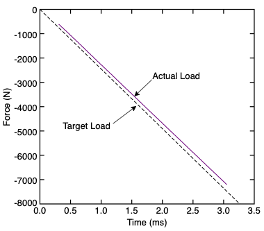
The following figure plots target and actual smoothed force for this simulation. The actual force lags behind the target force, but may actually be sufficient for this simulation. In other words, using just proportional control may be sufficient for many simulations. For other simulations, adding "I" and "D" may be needed. Two examples are if the lag expected in proportional control in unacceptable or if activation of evolving [math]\displaystyle{ A_t }[/math] causes proportional control to deteriorate from well-controlled simulations.

Choose [math]\displaystyle{ K_i }[/math]

When actual force lags the target force in proportional control, the integrated error will increase. Adding gain related to integrated error can penalize that increase such that the lag is reduced. The next step is to keep (Kd)=0 but now increase (Ki) to reduce the integrated error. As (Ki) is increased, the integrated error will get smaller. As (Ki) gets larger, the control will likely to start to oscillate near the target force. If (Ki) is too large the oscillations will grow in magnitude and the simulation will be come unstable. If (Ki) is about right, the oscillations will remain small and may even decay with time. A good choice seems to be to select (Ki) below the region where oscillations grow in magnitude.

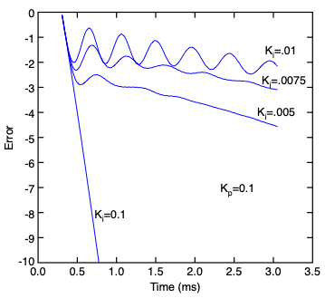
The following plot shows the integrated error (from archive file of results) for several values of (Ki) while keeping (Kp)=0.1. For (Ki)=0, the integrated error is large and continues to grow (plot is truncated at -10). As (Ki) increases, the integrated error gets smaller. When (Ki)=0.0075, some oscillations appear, but they die out with time. For (Ki)=0.01, the oscillations get large, but do not grow with time. For larger (Ki) (not shown), the oscillations grow and the simulation becomes unstable. For this example, (Ki)=0.01 was selected because it remains stable and it minimized the mean integrate error. Although oscillations are created, the goal of the next section is to remove them.

Choose [math]\displaystyle{ K_d }[/math]

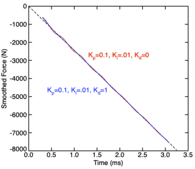
The addition of (Ki) reduced the lag, but caused force to oscillate around the target force. By adding gain related to error derivative, PID contral can suppress the oscillations. Again, increasing (Kd) damps the oscillations, but if it gets too high the simulation becomes unstable. Here using (Kd)=1 worked well.

The following plot commands smoothed force to target force for PI control alone (in red) and for PID control (in blue). The PI control oscillates around the target force. The PIC control is very close to target force with no oscillations.

Task Scheduling

In scripted files, a LoadControl custom task is scheduled with the following block:

CustomTask LoadControl
Parameter Load,(function)
... all remaining parameters with similar command

In XML files, these task options are scheduled using a <Schedule> element, which must be within the single <CustomTasks> block:

<Schedule name='LoadControl'>
   <Parameter name='Load'>(function)</Parameter>
   ... all remaining parameters with similar elements
</Schedule>